Every Prometheus metric is one of four types, and two of them — Counter and Gauge — are simple enough that most people get them right on instinct. The other two, Histogram and Summary, are where nearly every “why is my p95 alert lying to me” support thread eventually leads. This is the version that actually explains what’s happening underneath each type, not just when to reach for one.

Counter: only ever goes up

A Counter is a cumulative value that only increases — total HTTP requests served, total errors, total bytes sent. It resets to zero on process restart, and that reset is exactly why you almost never query a raw Counter value directly. Instead you wrap it in rate() or increase(), which are specifically designed to detect and correctly handle a counter reset — if the value goes down between two scrapes, Prometheus assumes a restart happened and adjusts the calculation rather than reporting a nonsensical negative rate.

rate(http_requests_total[5m])   # requests per second, averaged over 5 minutes

Gauge: a snapshot, can go either way

A Gauge represents a value at a point in time that can go up or down — current memory usage, current queue depth, current temperature, number of active connections right now. There’s no reset semantics to worry about because there’s no cumulative meaning to preserve; you query it directly, or apply functions like avg_over_time() or max_over_time() if you want a trend rather than an instantaneous read.

The single most common instrumentation mistake here is backwards: using a Gauge for something that should be a Counter (losing the ability to calculate a rate cleanly), or a Counter for something that should be a Gauge (current queue depth as an ever-incrementing counter makes no physical sense — a queue can shrink).

Histogram: buckets, and an approximate percentile

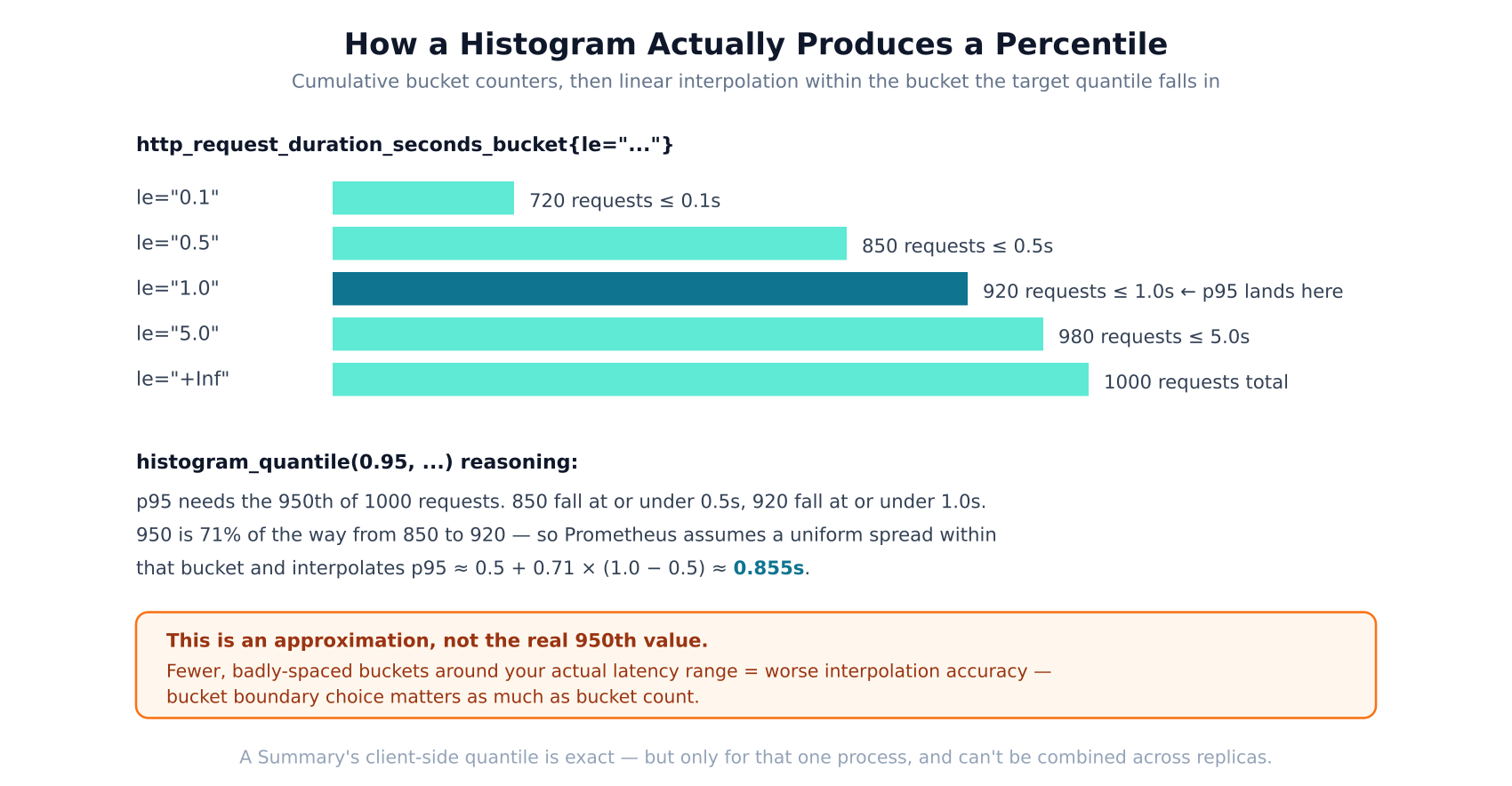
A Histogram samples observations — request durations, response sizes — and sorts them into configurable buckets, each with an upper bound (le, “less than or equal to”). Crucially, each bucket in Prometheus’s implementation is cumulative: the le="1.0" bucket count includes everything that also fell into le="0.5" and le="0.1". Under the hood, every bucket is just a Counter, plus a _sum (total of all observed values) and _count (total number of observations) — which is precisely why histograms aggregate cleanly across multiple instances: you’re just summing counters, something Prometheus is already good at.

Getting a percentile out of this requires the histogram_quantile() function, and it’s worth understanding that the result is a mathematical approximation: Prometheus finds which bucket the target percentile’s rank falls into, then linearly interpolates a value across that bucket’s range, assuming observations are spread evenly within it — which is rarely exactly true. This is also why bucket boundaries matter more than bucket count: five well-chosen buckets that bracket your actual latency distribution tightly will give a more accurate p95 than fifteen buckets poorly spaced relative to where your real traffic actually falls.

histogram_quantile(0.95, rate(http_request_duration_seconds_bucket[5m]))

The other practical cost: every bucket is its own time series. A histogram with 15 buckets across 20 services is 300 time series before you’ve added a single label — cardinality adds up fast, and it’s the main reason bucket boundaries should be chosen deliberately for the specific thing being measured, not copy-pasted defaults.

Summary: exact, but not aggregatable

A Summary calculates its quantiles client-side, inside the application process itself, using a sliding time window. The percentile it reports is genuinely exact for that one process’s own observations — no interpolation, no approximation. The catch, and it’s a significant one: a Summary’s calculated quantile cannot be meaningfully combined across multiple instances. Averaging three replicas’ individual p95 values doesn’t produce the fleet-wide p95 — it’s not how percentiles work mathematically, since a percentile isn’t a linear quantity you can average. If you’re running more than one instance of anything — which, in practice, is almost everything — this is usually the deciding factor against using a Summary.

What a Summary is genuinely good for: lower cardinality (no per-bucket time series, just the configured quantiles plus _sum/_count), and a workload where you specifically need an exact quantile for a single, non-replicated process and never need to combine it with anything else.

Instrumenting both, side by side

from prometheus_client import Counter, Gauge, Histogram, Summary

requests_total = Counter('http_requests_total', 'Total requests')
queue_depth    = Gauge('queue_depth', 'Current queued items')

request_latency_hist = Histogram(
    'http_request_duration_seconds',
    'Request latency',
    buckets=[0.05, 0.1, 0.25, 0.5, 1, 2.5, 5]
)

request_latency_summary = Summary(
    'http_request_duration_seconds_summary',
    'Request latency (single-instance exact quantile)'
)

Which one, by default

In practice: reach for Histogram as the default choice for latency and size measurements, specifically because it aggregates correctly the moment you have more than one replica — which you eventually will, even in a homelab, the day you split a service across two containers for the first time. Reach for Summary only when you’ve deliberately decided you need an exact, single-process quantile and genuinely never need to combine it with anything else. And keep Counter for anything that only accumulates, Gauge for anything that’s a live snapshot — get those two right, and the two harder types are just a question of whether aggregation across instances matters to you, which for almost everyone building anything beyond a single-process toy, it eventually does.